
Downloads: 1
Diff of
/README.md
[000000]
..
[87f2bb]
Switch to unified view
| a | b/README.md | ||
|---|---|---|---|
| 1 | |||
| 2 | # Medical Text Classification using Dissimilarity Space |
||
| 3 | |||
| 4 |  |
||
| 5 | |||
| 6 | ## Goal |
||
| 7 | |||
| 8 | This project goal is to develop a classifier that given a medical transcription text classifies its medical specialty. |
||
| 9 | |||
| 10 | **Note:** The goal of this project is not necessarily to achieve state-of-the-art results, but to try the idea of dissimilarity space for the task of text classification (see "main idea" section below). |
||
| 11 | |||
| 12 | ## Data |
||
| 13 | The original data contains 4966 records, each including three main elements: <br/> |
||
| 14 | |||
| 15 | **Transcription** - Medical transcription of some patient (text). <br/> |
||
| 16 | |||
| 17 | **Description** - Short description of the transcription (text). <br/> |
||
| 18 | |||
| 19 | **Medical Specialty** - Medical specialty classification of transcription (category). <br/> |
||
| 20 | |||
| 21 | The table below displays several examples: |
||
| 22 | |||
| 23 | | | Description | Transcription | Medical Specialty | |
||
| 24 | | --- | --- | --- | :----: | |
||
| 25 | | (1) |2-D M-Mode. Doppler.| 2-D M-MODE: , ,1. Left atrial enlargement with left atrial diameter of 4.7 cm.,2. Normal size right and left ventricle.,3. Normal LV systolic function with left ventricular ejection fraction of 51%.,4. Normal LV diastolic function.,5. No pericardial effusion.,6. Normal morphology of aortic valve, mitral valve, tricuspid valve, and pulmonary valve.,7. PA systolic pressure is 36 mmHg.,DOPPLER: , ,1. Mild mitral and tricuspid regurgitation.,2. Trace aortic and pulmonary regurgitation.|Cardiovascular / Pulmonary| |
||
| 26 | | (2) |AP abdomen and ultrasound of kidney.|EXAM: , AP abdomen and ultrasound of kidney.,HISTORY:, Ureteral stricture.,AP ABDOMEN ,FINDINGS:, Comparison is made to study from Month DD, YYYY. There is a left lower quadrant ostomy. There are no dilated bowel loops suggesting obstruction. There is a double-J right ureteral stent, which appears in place. There are several pelvic calcifications, which are likely vascular. No definite pathologic calcifications are seen overlying the regions of the kidneys or obstructing course of the ureters. Overall findings are stable versus most recent exam.,IMPRESSION: , Properly positioned double-J right ureteral stent. No evidence for calcified renal or ureteral stones.,ULTRASOUND KIDNEYS,FINDINGS:, The right kidney is normal in cortical echogenicity of solid mass, stone, hydronephrosis measuring 9.0 x 2.9 x 4.3 cm. There is a right renal/ureteral stent identified. There is no perinephric fluid collection.,The left kidney demonstrates moderate-to-severe hydronephrosis. No stone or solid masses seen. The cortex is normal.,The bladder is decompressed.,IMPRESSION:,1. Left-sided hydronephrosis.,2. No visible renal or ureteral calculi.,3. Right ureteral stent. |Radiology| |
||
| 27 | | (3) | Patient having severe sinusitis about two to three months ago with facial discomfort, nasal congestion, eye pain, and postnasal drip symptoms.|HISTORY:, I had the pleasure of meeting and evaluating the patient referred today for evaluation and treatment of chronic sinusitis. As you are well aware, she is a pleasant 50-year-old female who states she started having severe sinusitis about two to three months ago with facial discomfort, nasal congestion, eye pain, and postnasal drip symptoms. She states she really has sinus......| Allergy / Immunology| |
||
| 28 | |||
| 29 | |||
| 30 | There are 40 different categories. **Figure 1** displays the distribution of the top 20 categories in the dataset. |
||
| 31 | |||
| 32 | <br/> |
||
| 33 | |||
| 34 | | | |
||
| 35 | | --- | |
||
| 36 | | **Figure 1**: Top 20 categories| |
||
| 37 | |||
| 38 | |||
| 39 | One can see that the dataset is very unbalanced - most categories represent less than 5% of the total, each. <br/> |
||
| 40 | So we process the dataset as follows: |
||
| 41 | - Drop categories with less than 50 samples. |
||
| 42 | - Drop "general" categories (For example, the "Surgery" category is kind of a general category as there can be surgeries belonging to specializations like cardiology, neurology etc. ). |
||
| 43 | - Combine " Neurology" and " Neurosurgery" categories into a single category. |
||
| 44 | |||
| 45 | 12 categories remained, and we take the most common 5 categories to be the main data (see **Figure 2**). The rest left out for evaluation purposes (see point B at Evaluation section below). |
||
| 46 | |||
| 47 | The main data contains 1540 records, and is divided into 70% train set, 15% validation set, and 15% test set. |
||
| 48 | |||
| 49 | |||
| 50 | | 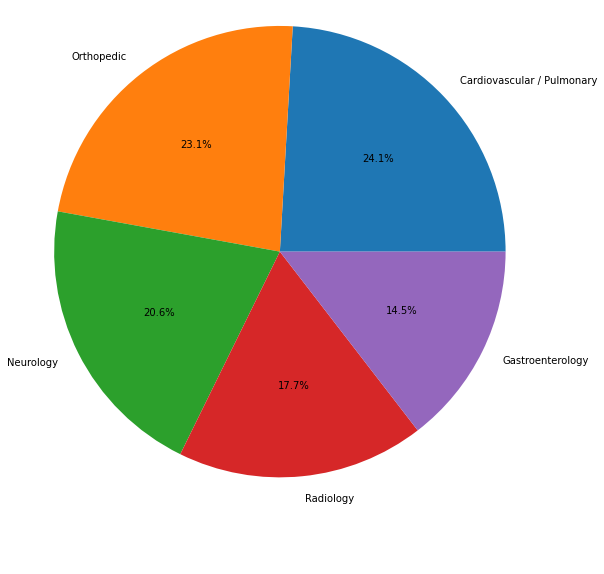| |
||
| 51 | | --- | |
||
| 52 | | **Figure 2**: Selected categories| |
||
| 53 | |||
| 54 | One can try either the descriptions or the transcriptions (or both) as the samples, but due to limitations in time and memory I use only the descriptions (see **Figure 3** and **Figure 4**, which displays the text lengths histograms). |
||
| 55 | |||
| 56 | |||
| 57 | | 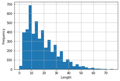 | 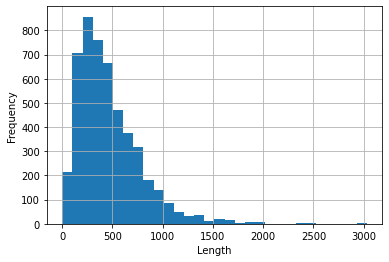 | |
||
| 58 | | --- | --- | |
||
| 59 | | **Figure 3**: Descriptions length histogram| **Figure 4**: Transcriptions length histogram| |
||
| 60 | |||
| 61 | |||
| 62 | ## Main Idea |
||
| 63 | The main idea used in this project is to learn a distance measure between the texts, and then use this measure to project the data into dissimilarity space. Then we train a classifier using the embedded vectors for predicting medical specialties. |
||
| 64 | |||
| 65 | This idea is adapted from the paper [Spectrogram Classification Using Dissimilarity Space][1] with some adjustments (detailed below) because in this project we are using textual data instead of images. |
||
| 66 | |||
| 67 | |||
| 68 | ## Scheme |
||
| 69 | The training procedure consists of several steps which are schematized in **Figure 5**. |
||
| 70 | |||
| 71 | | 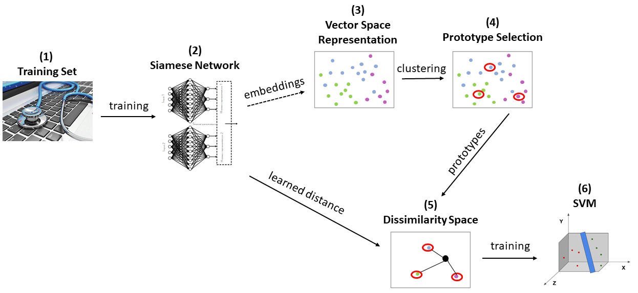 | |
||
| 72 | | --- | |
||
| 73 | | **Figure 5**: Training Scheme | |
||
| 74 | |||
| 75 | **(1) Training Set** <br/> |
||
| 76 | A customized data loader is built from the train set. It produces pairs of samples with a probability of 0.5 that both samples belong to the same category. |
||
| 77 | |||
| 78 | **(2) Siamese Neural Network (SNN) Training** <br/> |
||
| 79 | The purpose of this phase is to learn a distance measure d(x,y) by maximizing the similarity between couples of samples in the same category, while minimizing the similarity for couples in different categories. <br/> |
||
| 80 | Our siamese network model consists of several components: |
||
| 81 | |||
| 82 | - **Two identical twin subnetworks** <br/> |
||
| 83 | Two identical sub-network that share the same parameters and weights. Each subnetwork gets as input a text and outputs a feature vector which is designed to represent the text. I chose as a subnetwork a pre-trained Bert model (a huggingface model which trained on abstracts from PubMed and on full-text articles from PubMedCentral, see [here][2]) followed by a fine-tuning layers: 1D convolution layers and a FF layer. |
||
| 84 | - **Subtract Block** <br/> |
||
| 85 | Subtracting the output feature vectors of the subnetworks yields a feature vector that representing the difference between the texts: <br/> |
||
| 86 | |||
| 87 | - **Fully Connected Layer (FCL)** <br/> |
||
| 88 | The output vector of the subtract block is fed to the FCL which returns a dissimilarity value for the pair of texts in the input. Then a sigmoid function is applied to the dissimilarity value to convert it to a probability value in the range [0, 1]. |
||
| 89 | |||
| 90 | We use Binary Cross Entropy as the loss function. |
||
| 91 | |||
| 92 | **(3-4) Prototype Selection** <br/> |
||
| 93 | In this phase, K prototypes are extracted from the training set. As the autores of [1] stated, it is not practical to take every sample in the training as a prototype. Alternatively, m centroids for each category separately are computed by clustering technique. This reduces the prototype list from the size of the training sample (K=n) to K=m*C (C=number of categories). I chose K-means for the clustering algorithm. |
||
| 94 | |||
| 95 | In order to represent the training samples as vectors for the clustering algorithm, the authors in [1] used the pixel vector of each image. In this project, I utilize one of the subnetworks of the trained SNN to retrieve the feature vectors of every training sample (recall that the subnetwork gives us an embedded vector which represent the input text). |
||
| 96 | |||
| 97 | **(5) Projection in the Dissimilarity Space** <br/> |
||
| 98 | In this phase the data is projected into dissimilarity space. In order to obtain the representation of a sample x in the dissimilarity space, we calculate the similarity between the sample and the selected set of prototypes P=p1,...pk, which resulting in a dissimilarity vector: <br/> |
||
| 99 | F(x)=[d(x,p1),d(x,p2),...,d(x,pk)] <br/> |
||
| 100 | The similarity among a sample and a prototype d(x,p) is obtained using the trained SNN. |
||
| 101 | |||
| 102 | **(6) SVM Classifiers** <br/> |
||
| 103 | In this phase an ensemble of SVMs are trained using a One-Against-All approach: For each category an SVM classifier is trained to discriminate between this category and all the other categories put together. A sample is then assigned to the category that gives the highest confidence score. The inputs for the classifiers are the projected train data. |
||
| 104 | |||
| 105 | ## Evaluation |
||
| 106 | |||
| 107 | We evaluate the full procedure using the usual metrics (precision, recall, F1-score) on two left-out datasets: |
||
| 108 | |||
| 109 | **A) "Regular" test set** - This dataset includes texts that their categories appear in the train categories. We use this dataset in the following way: <br/> |
||
| 110 | - Projecti the test text samples into dissimilarity space using the trained SNN model and the prototype list we found during the training phase. |
||
| 111 | - Feed the projected test set into the trained SVM classifiers, and examine the results. |
||
| 112 | |||
| 113 | **B) "Unseen" test set** - this dataset includes texts that their categories **don't appear** in the train categories (hence the name "unseen"). We use this dataset to check whatever the trained SNN model can be utilized to measure the distance between texts that belong to "unseen" categories (and then, eventually, classify correctly their category). We check this in the following way: <br/> |
||
| 114 | - Split the "unseen" test set into train and test sets. |
||
| 115 | - Perform steps 3,4,5,6 in the training phase on the train set. Note that we don't train the SNN model agian. |
||
| 116 | - Predict the test set categories as we do in A). |
||
| 117 | |||
| 118 | We will mainly focus on A) for the evaluation. B) will be a bonus. |
||
| 119 | |||
| 120 | ## Results |
||
| 121 | |||
| 122 | **Figures 6** and **7** display the confusion matrix and the classification report for the test set and the "unseen" test set. |
||
| 123 | |||
| 124 | A high precision score for a category indicates that the classifier is usually accurate when detecting this category. |
||
| 125 | A high recall score for a category indicates that the classifier is able to detect many samples that belong to this category. |
||
| 126 | F1 score is the harmonic mean of precision and recall scores. |
||
| 127 | |||
| 128 | |  | 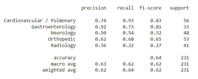| |
||
| 129 | | --- | --- | |
||
| 130 | | **Figure 6**: "Regular" test set results. | |
||
| 131 | |||
| 132 | It can be seen that the overall F1-score for the "regular" test set is quite low - 0.64. Some categories got relatively high results on some scores (for example "Gastroenterology" precision score is 0.92 and F1 score is 0.83). But for most of the categories we got poor results. |
||
| 133 | |||
| 134 | It is interesting to see from the confusion matrix that in many cases the classifier mistakenly classifies "Neurology" instead of "Orthopedic" and vice versa. One possible explanation is that these two categories overlap to some extent. For example some orthopedic issues usually involve the nervous system (spine problems etc.). |
||
| 135 | |||
| 136 | Another nore is that it seems that the "Radiology" category is also a "super-category", since in many cases the classifier outputs "Radiology" instead of other categories, and vice versa. It makes sense since every medical specialty may require medical imaging tests such as CT and MRI in order to perform a diagnosis to the patient. |
||
| 137 | |||
| 138 | | 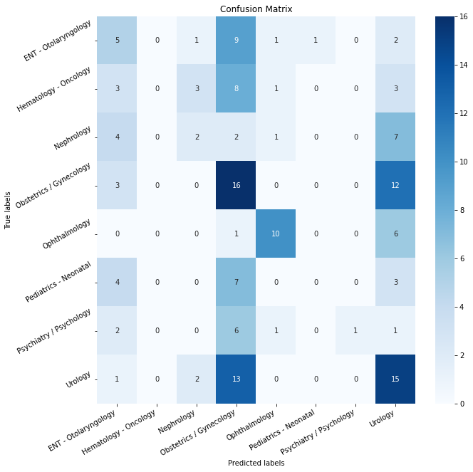 | 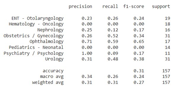| |
||
| 139 | | --- | --- | |
||
| 140 | | **Figure 7**: "Unseen" test set results. | |
||
| 141 | |||
| 142 | The results for the "unseen" set are very low, suggesting the model has not been generalized to other categories. |
||
| 143 | |||
| 144 | ## Further Analysis |
||
| 145 | |||
| 146 | In this section we attempt to analyze the results further. |
||
| 147 | |||
| 148 | **Figure 8** shows for the siamese neural network its train and validation losses per epoch. |
||
| 149 | | 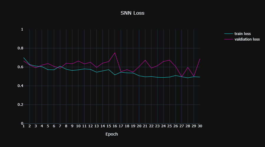 | |
||
| 150 | | --- | |
||
| 151 | | **Figure 8:** | |
||
| 152 | |||
| 153 | It can be seen that the network achieved a train loss around 0.5 in 30 epochs, that the validation loss is unstable, and that the rate of the learning is quite slow. We can try to improve these issues by playing with the hyperparameters of the SNN model (learning rate, batch size, architecture etc.). The "TODO" section below elaborates the possible options. |
||
| 154 | |||
| 155 | **Figure 9** displays the similarity scores per batch in the training set, by the following way: For each batch we calculate the average similarity score of pairs that belong to the same category ("matching categories") , and calculate separately the average similarity score of pairs that belong to different categories ("unmatching categories"). **Figure 10** displays the same but for the validation set. |
||
| 156 | |||
| 157 | |  | 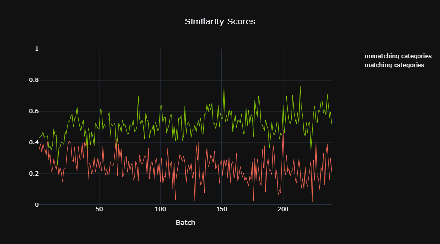| |
||
| 158 | | --- | --- | |
||
| 159 | | **Figure 9:** Similarity Scores, training set. | **Figure 10:** Similarity Scores, validation set.| |
||
| 160 | |||
| 161 | It can be seen that the range of similarity scores for texts belonging to the same category is different from the range of texts belonging to different categories, and that the first range is higher. So it appears that the SNN model managed to learn a distance measure between the texts. |
||
| 162 | |||
| 163 | |||
| 164 | **Figure 11** displays the training set after we projected it twice: first by doing phase (3) of the training scheme, and the second by applying PCA in order to display it in 3D. |
||
| 165 | |||
| 166 | | 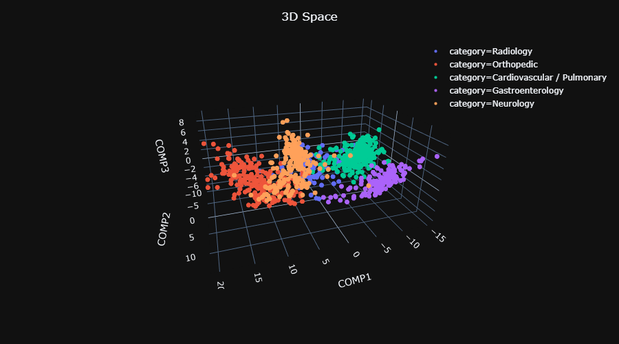 | |
||
| 167 | | --- | |
||
| 168 | | **Figure 11**: **Embedded train data** by using the trained SNN model. This figure displays its projection into a 3D space using PCA. Explained variance: 93% | |
||
| 169 | |||
| 170 | We can see that there is an impressive separation between the categories. In addition there is an overlap between the categories "Neurology" and "Orthopedic", and overlap between the "Radiology" category and all others, as we expected from the results. |
||
| 171 | |||
| 172 | Note that it seems that one could use this projected data and train directly the classifier on it instead of projecting the data into dissimilarity space. |
||
| 173 | |||
| 174 | **Figure 12** displays the projection into the dissimilarity space of the "regular" train and test sets (A and B plots), and of the "unseen" train and test sets (C and D plots). As we did in Figure 11, we used PCA to display the projection in 3D. |
||
| 175 | |||
| 176 | | | | |
||
| 177 | | --- | --- | |
||
| 178 | | | | |
||
| 179 | |**A:** Regular train set. Explained variance: 91% |**B:** Regular test set. Explained variance: 89% | |
||
| 180 | |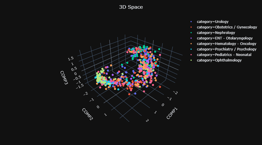 | | |
||
| 181 | |**C:** "Unseen" train set. Explained variance: 88% | **D:** "Unseen" test set. Explained variance: 89%| |
||
| 182 | |||
| 183 | It seems that the projection of the "regular" train and test set is quite meaningful, but the projection of the "unseen" train and test is not. |
||
| 184 | |||
| 185 | |||
| 186 | ## Libaries |
||
| 187 | Pytorch, HuggingFace, sklearn, numpy, Plotly |
||
| 188 | |||
| 189 | ## Resources |
||
| 190 | |||
| 191 | [1] "Spectrogram Classification Using Dissimilarity Space" (https://www.mdpi.com/2076-3417/10/12/4176/htm) |
||
| 192 | |||
| 193 | [2] "PubMedBERT (abstracts + full text)" https://huggingface.co/microsoft/BiomedNLP-PubMedBERT-base-uncased-abstract-fulltext |
||
| 194 | |||
| 195 | [1]: https://www.mdpi.com/2076-3417/10/12/4176/htm "Spectrogram Classification Using Dissimilarity Space" |
||
| 196 | |||
| 197 | [2]: https://huggingface.co/microsoft/BiomedNLP-PubMedBERT-base-uncased-abstract-fulltext "PubMedBERT (abstracts + full text)" |
||
| 198 | |||
| 199 |