---
title: "ondisk"
output:
html_document:
toc: true
toc_float:
collapsed: false
smooth_scroll: false
---
```{css, echo=FALSE}
.watch-out {
color: black;
}
```
```{r setup, include=FALSE}
# use rmarkdown::render_site(envir = knitr::knit_global())
knitr::opts_chunk$set(highlight = TRUE, echo = TRUE)
```
## Import VisiumHD Data
We first have to download some packages that are necessary to import datasets from `.parquet` and `.h5` files provided by the VisiumHD readouts.
```{r class.source="watch-out", eval = FALSE}
install.packages("arrow")
BiocManager::install("rhdf5")
library(arrow)
library(rhdf5)
```
We use the **importVisiumHD** function to start analyzing the data. The data has 393401 spots which we will use OnDisk-backed methods to efficiently manipulate, analyze and visualize these spots.
The VisiumHD readouts provide multiple bin sizes which are aggregated versions of the original 2$\mu$m $x$ 2$\mu$m capture spots. The default bin sizes are **(i)** 2$\mu$m $x$ 2$\mu$m, **(ii)** 8$\mu$m $x$ 8$\mu$m and **(iii)** 16$\mu$m $x$ 16$\mu$m.
```{r class.source="watch-out", eval = FALSE}
hddata <- importVisiumHD(dir.path = "VisiumHD/outs/",
bin.size = "8",
resolution_level = "hires")
```
## Saving/Loading VoltRon Objects
We use **BPCells** and **ImageArray** packages to accelerate operations of feature matrices and images. Here **BPCells** allows users access and operate on large feature matrices or clustering/spatial analysis, while **ImageArray** provides [pyramids images](https://en.wikipedia.org/wiki/Pyramid_(image_processing)) to allow fast access to large microscopy images. You can download these package from GitHub using **devtools**.
```{r class.source="watch-out", eval = FALSE}
devtools::install_github("bnprks/BPCells/r")
devtools::install_github("BIMSBbioinfo/ImageArray")
library(BPCells)
library(ImageArray)
```
We can now save the VoltRon object to disk, large matrices and images will be written to either **hdf5** or **zarr** files depending on the **format** arguement, and the rest of the R object would be written to an `.rds` file, both under the designated **output**.
```{r class.source="watch-out", eval = FALSE}
hddata <- saveVoltRon(hddata, format = "HDF5VoltRon", output = "data/VisiumHD")
```
If you want you can load the VoltRon object from the same path as you have saved.
```{r class.source="watch-out", eval = FALSE}
hddata <- loadVoltRon("data/VisiumHD/")
```
## Cell/Spot Analysis
The **BPCells** package provides fast methods to achieve operations common to single cell analysis such as filtering, normalization and dimensionality reduction. Here we have an example of single-cell like clustering of VisiumHD bins which is efficiently clustered.
```{r class.source="watch-out", eval = FALSE}
spatialpoints <- vrSpatialPoints(hddata)[as.vector(Metadata(hddata)$Count > 10)]
hddata <- subset(hddata, spatialpoints = spatialpoints)
hddata <- normalizeData(hddata, sizefactor = 10000)
hddata <- getFeatures(hddata, n = 3000)
selected_features <- getVariableFeatures(hddata)
hddata <- getPCA(hddata, features = selected_features, dims = 30)
hddata <- getUMAP(hddata, dims = 1:30)
```
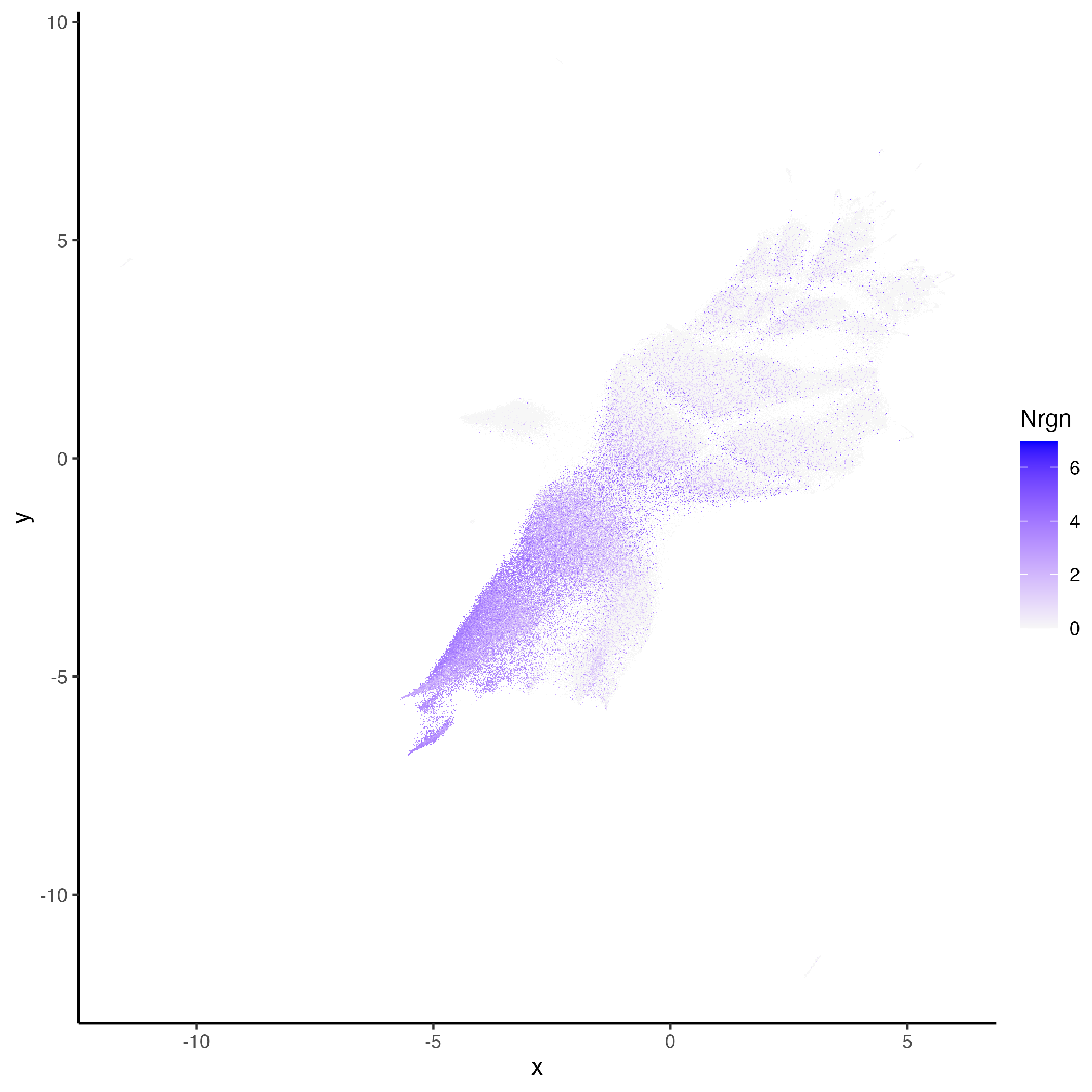
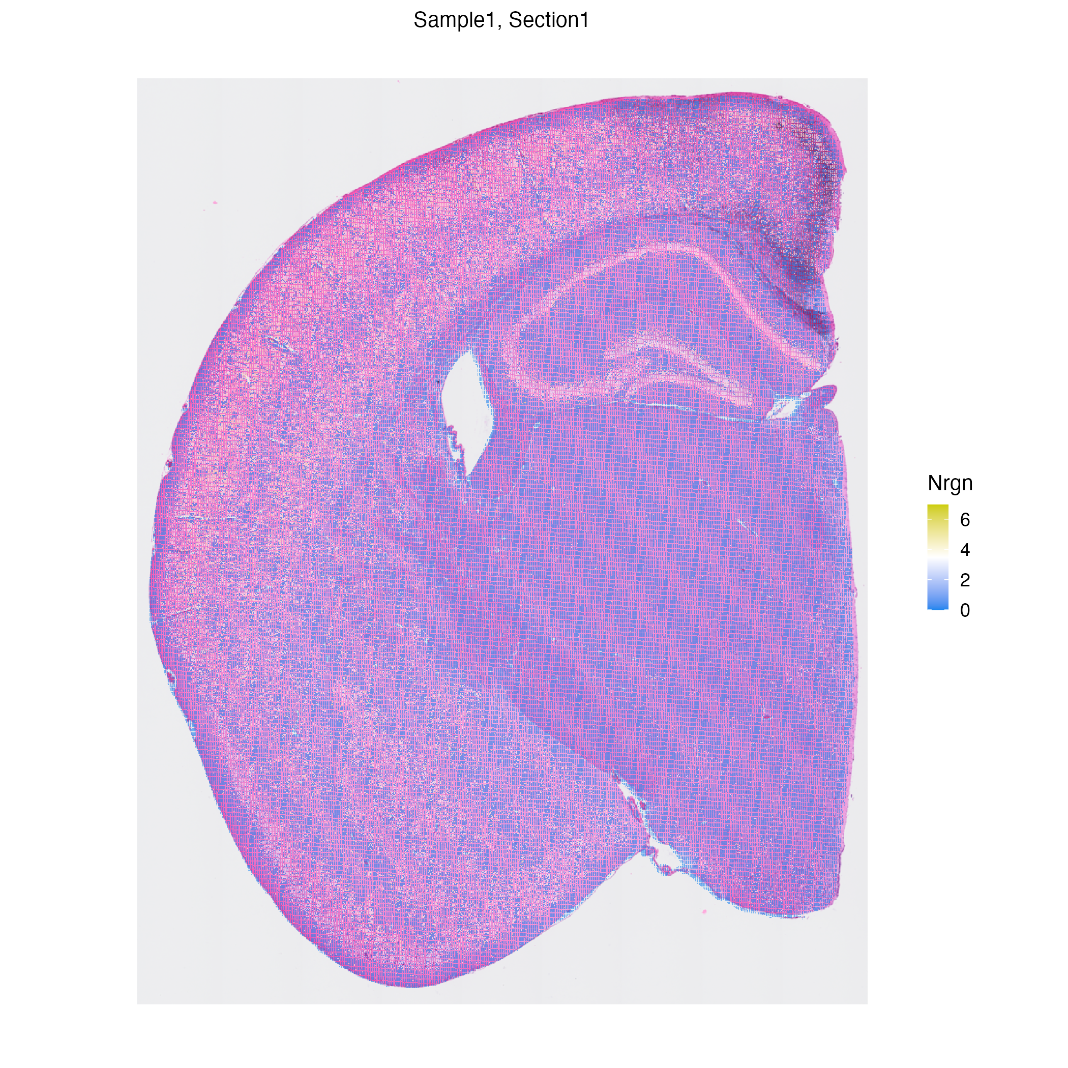
We can now visualized genes over embedding or spatial plots.
```{r class.source="watch-out", eval = FALSE}
vrEmbeddingFeaturePlot(hddata, features = "Nrgn", embedding = "umap")
vrSpatialFeaturePlot(hddata, features = "Nrgn")
```
## Spatial Data Alignment
The image registration workflow in the [Spatial Data Alignment](registration.html) tutorial can also be conducted using disk-backed methods of the VoltRon package.
```{r class.source="watch-out", eval = FALSE}
library(VoltRon)
Xen_R1 <- importXenium("Xenium_R1/outs", sample_name = "XeniumR1", resolution_level = 3)
Xen_R1_image <- importImageData("Xenium_FFPE_Human_Breast_Cancer_Rep1_he_image.tif",
sample_name = "XeniumR1image",
image_name = "H&E")
```
We can save both Xenium and H&E (image) datasets to disk before using the mini Shiny app for registration
```{r class.source="watch-out", eval = FALSE}
Xen_R1_disk <- saveVoltRon(Xen_R1,
format = "HDF5VoltRon",
output = "data/Xen_R1_h5", replace = TRUE)
Xen_R1_image_disk <- saveVoltRon(Xen_R1_image,
format = "HDF5VoltRon",
output = "data/Xen_R1_image_h5", replace = TRUE)
```
These disk-based datasets can then be loaded from the disk easily.
```{r class.source="watch-out", eval = FALSE}
Xen_R1_disk <- loadVoltRon("../data/OnDisk/Xen_R1_h5/")
Xen_R1_image_disk <- loadVoltRon("../data/OnDisk/Xen_R1_image_h5/")
```
VoltRon stores large images as pyramids to increase interactive visualization efficiency. This storage strategy allows shiny apps to zoom in to tissue niches in a speedy fashion. VoltRon incorporates `Image_Array` objects (https://github.com/BIMSBbioinfo/ImageArray) to define these pyramids.
```{r class.source="watch-out", eval = FALSE}
vrImages(Xen_R1_image_disk, as.raster = TRUE)
```
```
Image_Array Object
Series 1 of size (3,27587,20511)
Series 2 of size (3,13794,10256)
Series 3 of size (3,6897,5128)
Series 4 of size (3,3449,2564)
Series 5 of size (3,1725,1282)
Series 6 of size (3,863,641)
Series 7 of size (3,432,321)
```
We can now visualize and align the Xenium and H&E objects.
```{r class.source="watch-out", eval = FALSE}
# Align spatial data
xen_reg <- registerSpatialData(object_list = list(Xen_R1_disk, Xen_R1_image_disk))
```
```{r class.source="watch-out", eval = FALSE}
# transfer aligned H&E to Xenium data
Xenium_reg <- xen_reg$registered_spat[[2]]
vrImages(Xen_R1_disk[["Assay1"]], name = "main", channel = "H&E") <- vrImages(Xenium_reg, name = "H&E_reg")
# visualize
vrImages(Xen_R1_disk, channel = "H&E", scale.perc = 10)
```