
Image Credit: https://www.biochain.com/nanostring-geomx-digital-spatial-profiling/
The [Nanostring's GeoMx Digital Spatial Profiler](https://nanostring.com/products/geomx-digital-spatial-profiler/geomx-dsp-overview/) is a high-plex spatial profiling technology which produces segmentation-based protein and RNA assays. The instrument allows users to select regions of interest (ROIs) from fluorescent microscopy images that capture the morphological context of the tissue. These are ROIs are then used to generate transcriptomic or proteomic profiles. We will import the ROI profiles generated from the GeoMx scan area where COVID-19 lung tissues were fitted into. See [GSE190732](https://www.ncbi.nlm.nih.gov/geo/query/acc.cgi?acc=GSE190732) for more information on this study. Here is the usage of **importGeoMx** function and necessary files for this example:| Argument | Description | Link |
|---|---|---|
| dcc.path | The path to DCC files directory | DDC files |
| pkc.file | GeoMx™ DSP configuration file | Human RNA Whole Transcriptomic Atlas for NGS |
| summarySegment | Segment summary table (.xls or .csv) | ROI Metadata file |
| image | The Morphology Image of the scan area | Image file |
| ome.tiff | The OME.TIFF Image of the scan area | OME.TIFF file |
| The OME.TIFF Image XML file | OME.TIFF (XML) file |
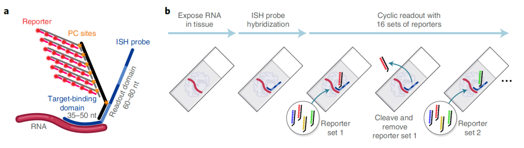
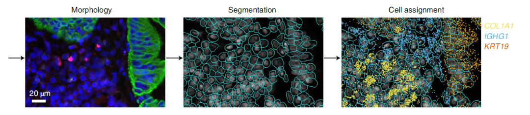
Image Credit: https://www.biorxiv.org/content/10.1101/2021.11.03.467020v1.full
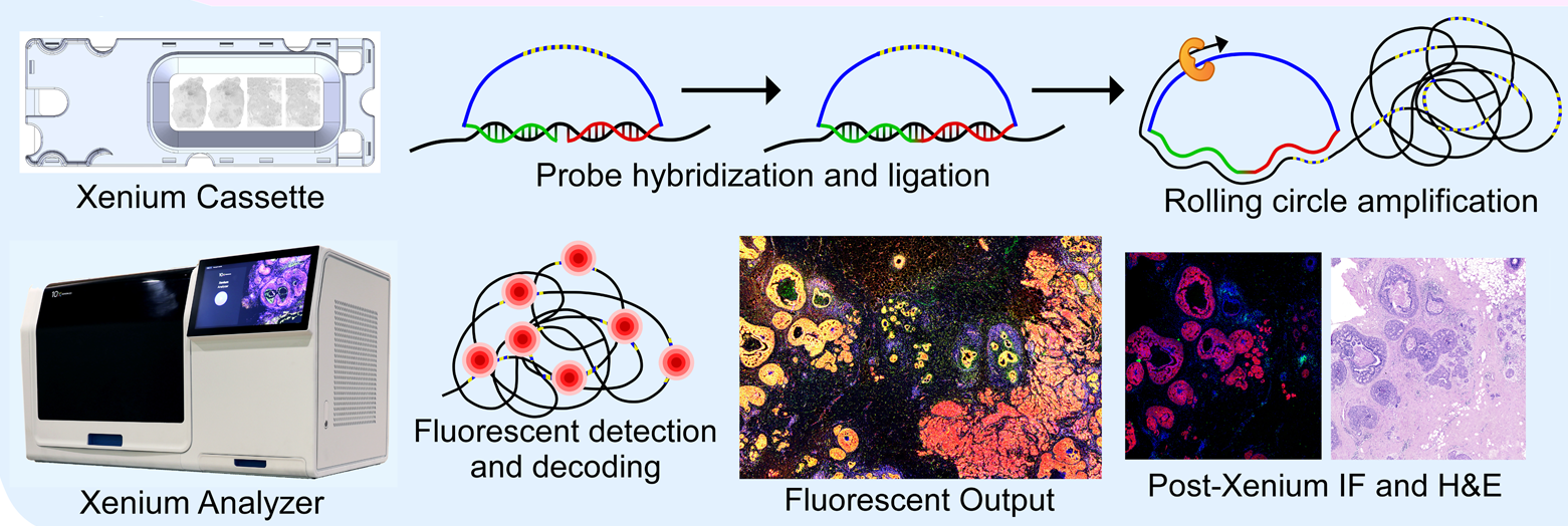
The [Nanostring's CosMx Spatial Molecular Imaging](https://nanostring.com/products/cosmx-spatial-molecular-imager/cosmx-smi-single-cell-imaging-de/) platform is a high-plex spatial multiomics technology that captures the spatial localization of both (i) transcripts from thousands of genes as well as (ii) the single cells with transcriptomic and proteomic profiles. We will use the readouts from two slides of a single CosMx experiment. You can download the data from the [Nanostring website](https://nanostring.com/products/cosmx-spatial-molecular-imager/ffpe-dataset/cosmx-smi-mouse-brain-ffpe-dataset/). We use the **importCosMx** function to import the CosMx readouts and create a VoltRon object. Here, we point to the folder of the [TileDB](https://tiledb.com/) array that stores feature matrix as well as the transcript metadata. ```{r eval = FALSE, class.source="watch-out"} CosMxR1 <- importCosMx(tiledbURI = "MuBrainDataRelease/") ``` ``` VoltRon Object Slide1: Layers: Section1 Slide2: Layers: Section1 Assays: CosMx(Main) ``` You can use the **import_molecules** argument to import positions and features of the transcripts along with the single cell profiles. ```{r eval = FALSE, class.source="watch-out"} CosMxR1 <- importCosMx(tiledbURI = "MuBrainDataRelease/", import_molecules = TRUE) ``` ## STOmics (MGI)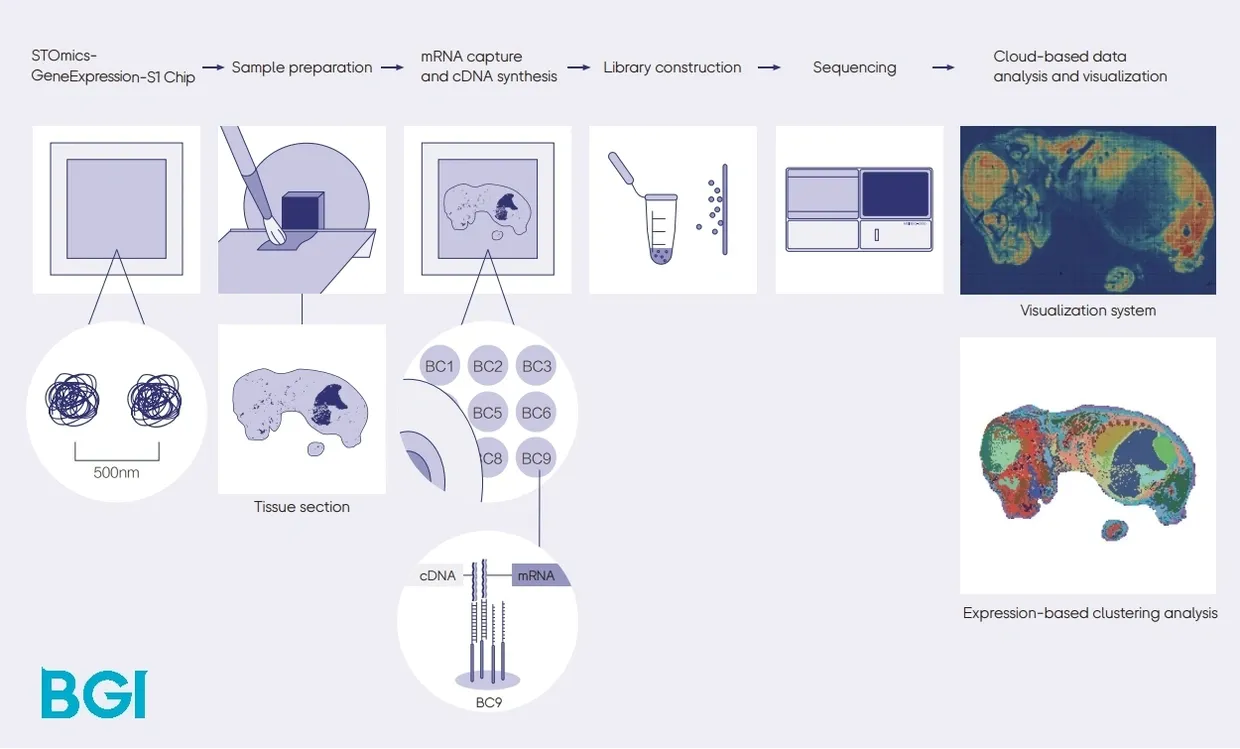
Image Credit: https://bgi-australia.com.au/stomics
Before importing the STOmics data to VoltRon, we first convert STOmics readouts to an h5ad file using the **stereopy** Python module. For more information, visit [https://stereopy.readthedocs.io/](https://stereopy.readthedocs.io/en/latest/Tutorials/Format_Conversion.html). See [here](https://stereopy.readthedocs.io/en/latest/content/00_Installation.html) for instructions on how to install **stereopy**. ```{python class.source="watch-out", eval = FALSE} import stereo as st import warnings warnings.filterwarnings('ignore') # read the GEF file data_path = './SS200000135TL_D1.tissue.gef' data = st.io.read_gef(file_path=data_path, bin_size=50) data.tl.raw_checkpoint() # remember to set flavor as scanpy adata = st.io.stereo_to_anndata(data, flavor='scanpy', output='sample.h5ad') ```We use the **importSTOmics** function to import the STOmics readouts and create a VoltRon object. Here, we point to the folder an h5ad file generated using the **stereo.io.stereo_to_anndata** method previously. ```{r eval = FALSE, class.source="watch-out"} vrdata <- importSTOmics(h5ad.path = "sample.h5ad") ``` ``` VoltRon Object Sample1: Layers: Section1 Assays: STOmics(Main) ``` ## GenePS (Spatial Genomics)
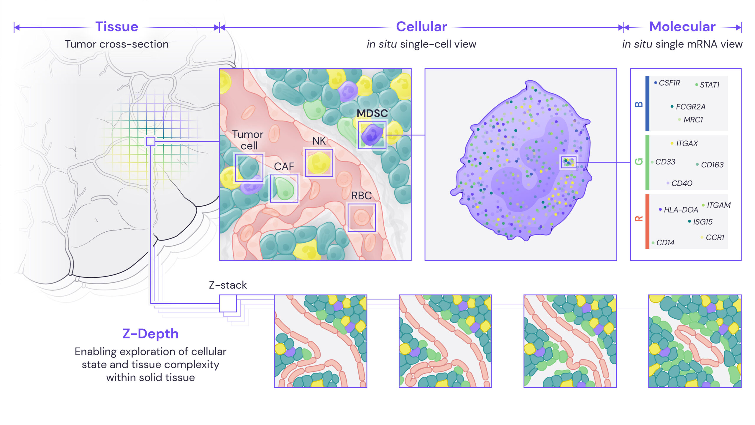
Image Credit: https://spatialgenomics.com/applications/
We use the **importGenePS** function to import the GenePS ([Spatial Genomics](https://spatialgenomics.com/product/)) readouts and create a VoltRon object. You can use the **import_molecules** argument to import positions and features of the transcripts along with the single cell profiles. The **resolution_level** argument determines the resolution of the DAPI image generated from the TIFF file. ```{r eval = FALSE, class.source="watch-out"} vrdata <- importGenePS(dir.path = "out/", import_molecules = TRUE, resolution_level = 7) ``` ``` VoltRon Object Sample1: Layers: Section1 Assays: GenePS(Main) GenePS_mol ``` ## PhenoCycler (Akoya)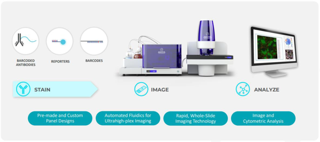
Image Credit: https://tep.cancer.illinois.edu/phenocycler-fusion-system/
We use the **importPhenoCycler** function to import the PhenoCycler ([Akoya Biosciences](https://www.akoyabio.com/)) readouts and create a VoltRon object. The function supports multiple readouts types depending on how the readouts were generated, this is controlled by the **type** arguement. For more information on all arguements of the function, see **help(importPhenoCycler)**. We used the Human FFPE tonsil tissue example with 83000 cells which could be found [here](https://akoya.app.box.com/s/lqaz1eyefni57sfynveh03e9sdy4aeuk). You have to download the contents and **dir.path** arguement should be set to the location of the **Example-dataset-for-MAV** folder. ```{r eval = FALSE, class.source="watch-out"} vr_pheno <- importPhenoCycler(dir.path = "Example-dataset-for-MAV/", type = "processor", sample_name = "Tonsil18AB") ``` ``` VoltRon Object Tonsil18AB: Layers: Section1 Assays: PhenoCycler(Main) ``` ## OpenST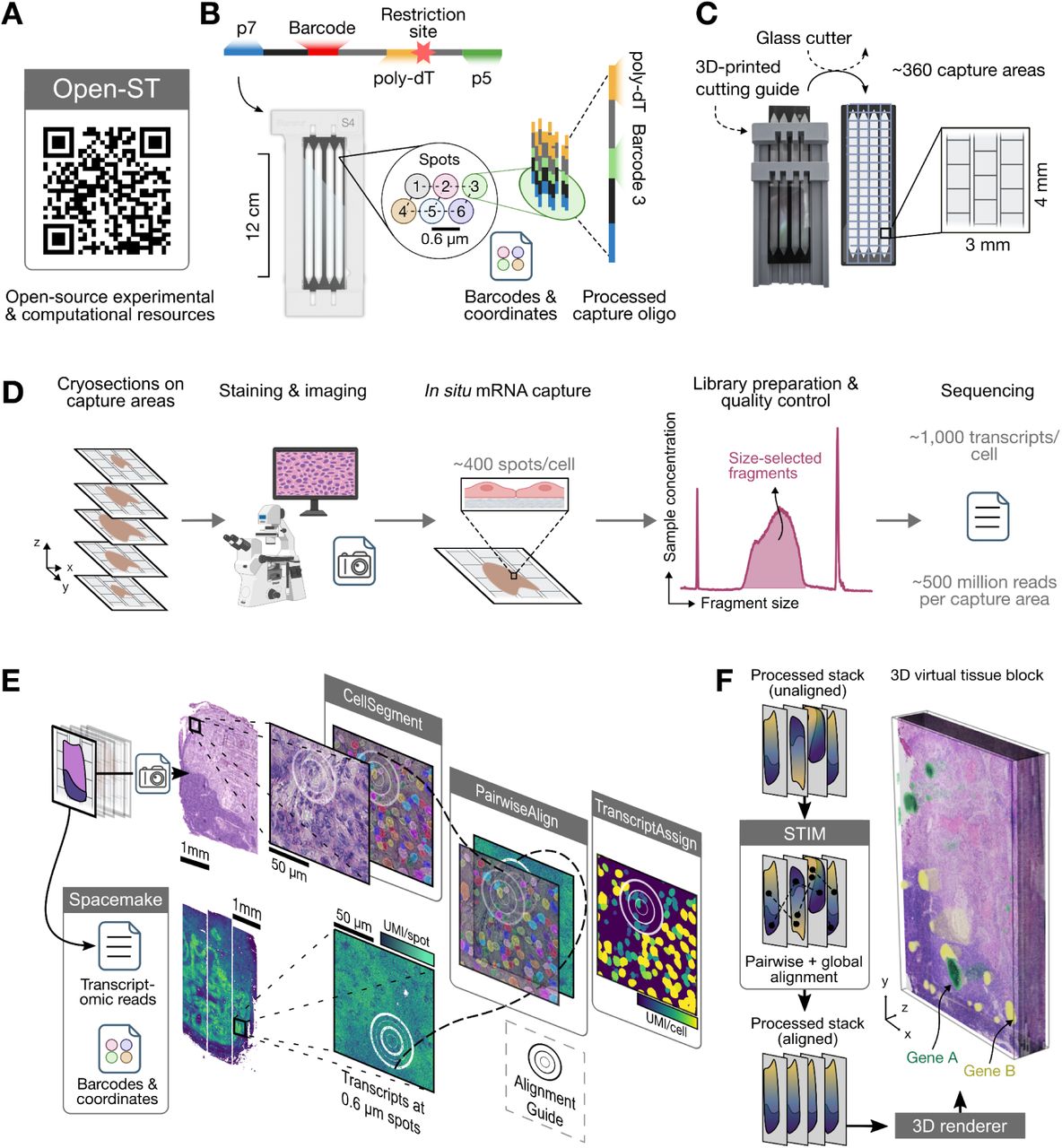
Image Credit: https://www.cell.com/cell/fulltext/S0092-8674(24)00636-6
We use the **importOpenST** function to import the OpenST [https://rajewsky-lab.github.io/openst/latest/](https://rajewsky-lab.github.io/openst/latest/) readouts and create a VoltRon object. The function will parse each section from the output h5ad file, define it as an independent assay in a single layer where these layers are ordered in a single tissue block. We use the metastatic lymph node example that is deposited to NCBI/GEO ([GSE251926](https://www.ncbi.nlm.nih.gov/geo/query/acc.cgi?acc=GSE251926)). Please use the **GSE251926_metastatic_lymph_node_3d.h5ad.gz** file and unzip it to use the importOpenST function below. ```{r eval = FALSE, class.source="watch-out"} vr_openst <- importOpenST(h5ad.path = "GSE251926_metastatic_lymph_node_3d.h5ad", sample_name = "MLN_3D") ``` ``` VoltRon Object MLN_3D: Layers: Section1 Section2 Section3 Section4 Section5 Section6 Section7 Section8 Section9 Section10 Section11 Section12 Section13 Section14 Section15 Section16 Section17 Section18 Section19 Assays: OpenST(Main) ``` ## DBIT-Seq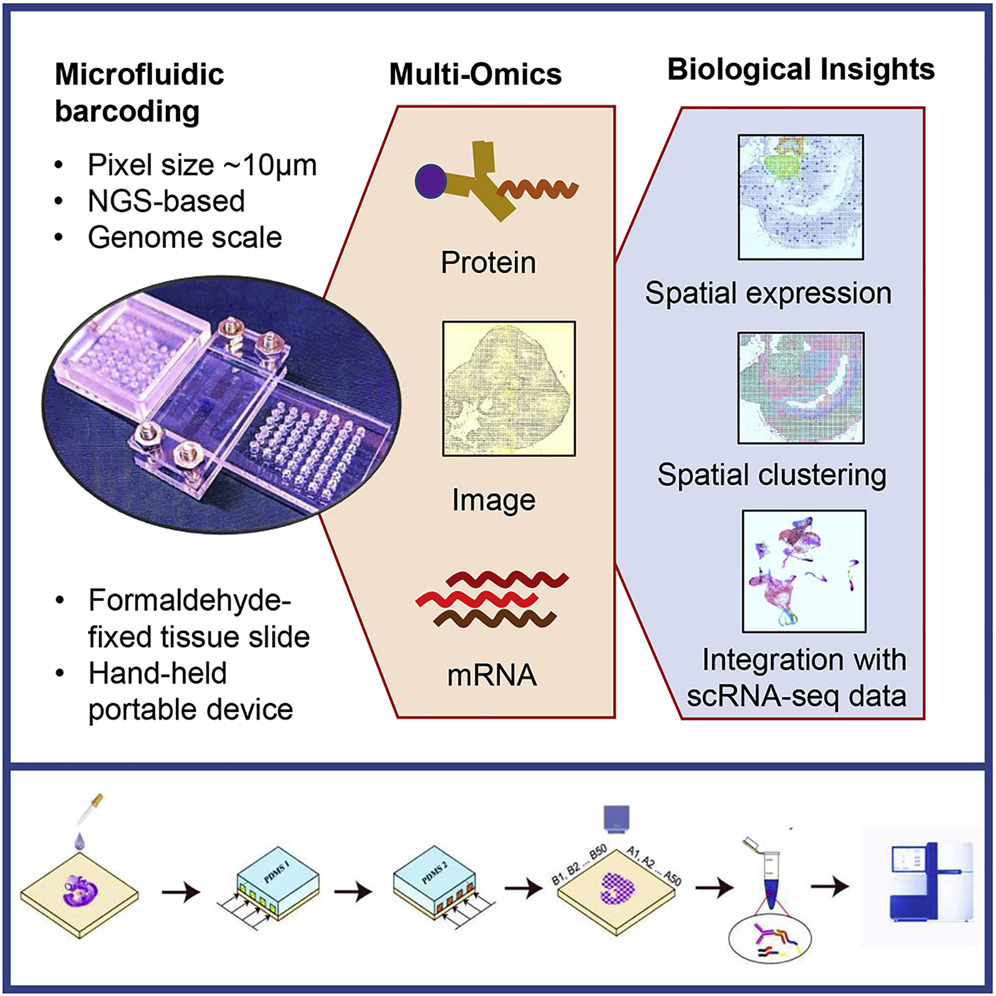
Image Credit: https://www.cell.com/cell/fulltext/S0092-8674(20)31390-8
We use the **importDBITSeq** function to import the DBIT-Seq [https://www.cell.com/cell/fulltext/S0092-8674(20)31390-8](https://www.cell.com/cell/fulltext/S0092-8674(20)31390-8) readouts and create a VoltRon object. The default path to the rna count matrix is accompanied by the path to the protein count matrix, which is optional. The **size** parameter here determines the size of each square pixel on the DBIT-Seq slide (default is 10$\mu$m). We use the example with developing eye field in a E10 mouse embryo using 10-μm microfluidic (sample id: 0719cL for RNA, and 0719aL for Protein) channels that is deposited to NCBI/GEO ([GSE137986](https://www.ncbi.nlm.nih.gov/geo/query/acc.cgi?acc=GSE137986)). ```{r eval = FALSE, class.source="watch-out"} vr_dbit <- importDBITSeq(path.rna = "GSM4189615_0719cL.tsv", path.prot = "GSM4202309_0719aL.tsv", size = 10, sample_name = "E10_Eye_2", image_name = "main") ``` ``` VoltRon Object E10_Eye_2: Layers: Section1 Assays: DBIT-Seq-RNA(Main) DBIT-Seq-Prot ``` ## ST data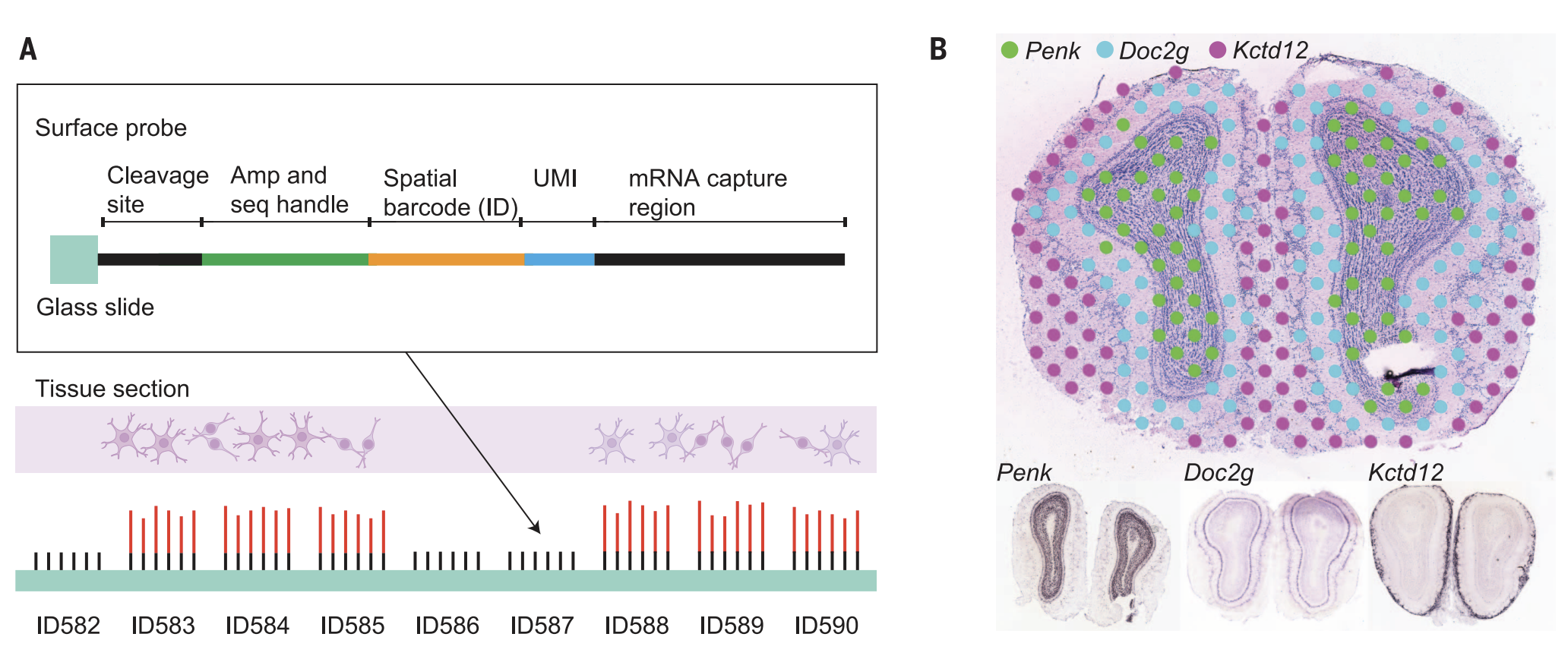
Image Credit: Ståhl, et. al (2016). Visualization and analysis of gene expression in tissue sections by spatial transcriptomics. Science, 353(6294), 78-82.
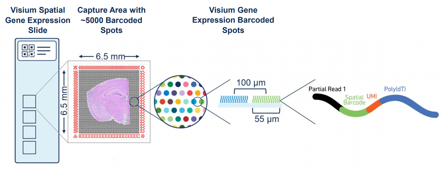
We demonstrate importing the original Spatial Transcriptomics (ST) datasets by formulating custom spot-level spatial transcriptomics datasets. We will use the **formVoltRon** function directly. We use the example provided by the [https://doi.org/10.5281/zenodo.4751624](https://doi.org/10.5281/zenodo.4751624). For more information you can also check the paper [here](https://www.ncbi.nlm.nih.gov/pmc/articles/PMC8516894/). We first import and manipulate count matrices and spot coordinates from the provided output files. Here we only demonstrate building a custom spot-level VoltRon object for the section "A1", however the remaining sections can be imported using the same method. ```{r eval = FALSE, class.source="watch-out"} # count matrix raw.data <- read.table("A1.tsv", header = TRUE, sep = "\t") spatialentities <- raw.data$X raw.data <- raw.data[,-1] raw.data <- t(as.matrix(raw.data)) # coords coords <- read.table("A1_selection.tsv", header = TRUE, sep = "\t") rownames(coords) <- paste(coords$x, coords$y, sep = "x") coords <- coords[entities,] coords <- coords[,c("pixel_x", "pixel_y")] colnames(coords) <- c("x", "y") ``` The image can be imported using the **magick** package. ```{r eval = FALSE, class.source="watch-out"} library(magick) img <- magick::image_read("HE/A1.jpg") img_info <- magick::image_info(img) ``` Before we form the VoltRon object, we should define the parameters for spot-level datasets. Here, we provide * the radius of a spot in the physical space (i.e. **spot.radius**) * the radius of a spot for visualization (i.e. **vis.spot.radius**) * The distance to the nearest spot, to be used for spatial neighborhood calculation (i.e. **nearestpost.distance**) The scaling parameter (scale_param) is required to overlay localization and distances of spots to the coordinate system of the imported image. Here, * the width of a ST slide is of 6200$\mu$m, * the diameter of a spot is 100$\mu$m (hence a radius of 50$\mu$m) and * the center-to-center distance between two spots is 200$\mu$m. * Each spot has at most 8 neighboring spots including vertically, horizontally and diagonally adjacent spots. ```{r eval = FALSE, class.source="watch-out"} scale_param <- img_info$width/6200 params <- list( spot.radius = 50*(scale_param), vis.spot.radius = 100*(scale_param), nearestpost.distance = (200*sqrt(2) + 50)*scale_param ) ``` Now we can combine all components into a VoltRon object. We should also flip the coordinates of spots vertically after creating the object. ```{r eval = FALSE, class.source="watch-out"} # make voltron object stdata <- formVoltRon(data = datax, image = img, coords = coords, assay.type = "spot", params = params, sample_name = "A1") stdata <- flipCoordinates(stdata) ``` We can now visualize spots and the adjacency between these spots simultaneously. ```{r eval = FALSE, class.source="watch-out"} stdata <- getSpatialNeighbors(stdata, method = "radius") vrSpatialPlot(stdata, graph.name = "radius", crop = T) ```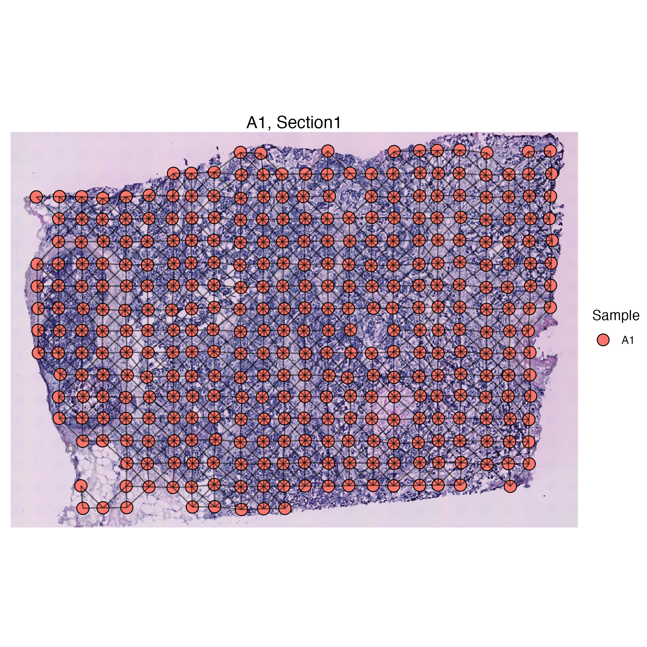
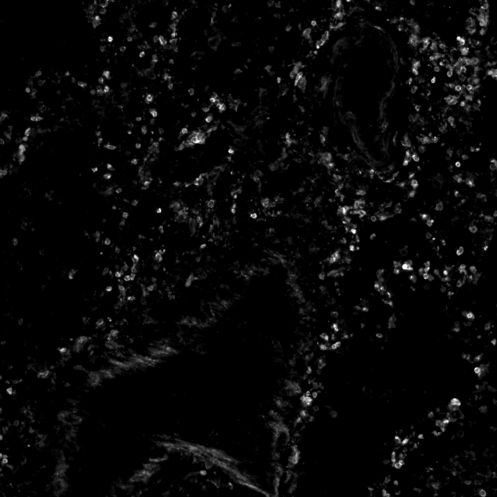
## Custom VoltRon objects VoltRon incorporates the **formVoltRon** function to assemble each component of a spatial omic assay into a VoltRon object. Here: * **the feature matrix**: the pxn feature to point matrix for raw counts and omic profiles * **metadata**: the metadata table * **image**: An image or a list of images with names associated to channel * **coordinates**: xy-Coordinates of spatial points * **segments**: the list of xy-Coordinates of each spatial point can individually be prepared before executing formVoltRon. We will use a single image based proteomic assay to demonstrate building custom VoltRon objects. Specifically, we use cells characterized by **multi-epitope ligand cartography (MELC)** with a panel of 44 parameters. We use the already segmented cells on which expression of **43 protein features** (excluding DAPI) were mapped to these cells. VoltRon also provides support for imaging based proteomics assays. In this next use case, we analyze cells characterized by **multi-epitope ligand cartography (MELC)** with a panel of 44 parameters. We use the already segmented cells on which expression of **43 protein features** (excluding DAPI) were mapped to these cells. You can download the files below [here](https://bimsbstatic.mdc-berlin.de/landthaler/VoltRon/ImportData/custom_vr_object.zip). ```{r eval = FALSE, class.source="watch-out"} library(magick) # feature x cell matrix intensity_data <- read.table("intensities.tsv", sep = "\t") intensity_data <- as.matrix(intensity_data) # metadata metadata <- read.table("metadata.tsv", sep = "\t") # coordinates coordinates <- read.table("coordinates.tsv", sep = "\t") coordinates <- as.matrix(coordinates) # image library(magick) image <- image_read("DAPI.tif") # create VoltRon object vr_object<- formVoltRon(data = intensity_data, metadata = metadata, image = image, coords = coordinates, main.assay = "MELC", assay.type = "cell", sample_name = "control_case_3", image_name = "DAPI") vr_object ``` ``` VoltRon Object control_case_3: Layers: Section1 Assays: MELC(Main) ``` VoltRon can store multiple images (or channels) associated with a single coordinate system. ```{r eval = FALSE, class.source="watch-out"} library(magick) image <- list(DAPI = image_read("DAPI.tif"), CD45 = image_read("CD45.tif")) vr_object<- formVoltRon(data = intensity_data, metadata = metadata, image = image, coords = coordinates, main.assay = "MELC", assay.type = "cell", sample_name = "control_case_3", image_name = "MELC") ``` These channels then can be interrogated and used as background images for spatial plots and spatial feature plots as well. ```{r eval = FALSE, class.source="watch-out"} vrImageChannelNames(vr_object) ``` ``` Assay Layer Sample Spatial Channels Assay1 MELC Section1 control_case_3 MELC DAPI,CD45 ``` You can extract each of these channels individually. ```{r eval = FALSE, class.source="watch-out"} vrImages(vr_object, name = "MELC", channel = "DAPI") vrImages(vr_object, name = "MELC", channel = "CD45") ```
 |
 |